Articles
June 28, 2022
How to Build a Transformer for Supervised Classification

# TensorFlow
# Supervised Learning
# Deep Learning
Learn how to implement a transformer in Python for supervised document classification in our series on using TensorFlow for supervised classification tasks.

Mehreen Saeed
In Transformers: What They Are and Why They Matter, I discussed the theory and the mathematical details behind how transformers work. This time I’ll show you how to build a simple transformer model for supervised classification tasks in Python using the APIs and objects from the Keras and TensorFlow libraries. We’ll work with the famous 20 newsgroup text dataset, which consists of around 18,000 newsgroup posts, classified into 20 topics. The goal is to learn which newsgroup belongs to which category/topic.
My goal is to show you how to build your own transformer model for classification, so we won’t perform any sophisticated or complex preprocessing or fine-tuning of the model to beat the performance of other methods on the same task. It is also important to note that the output shown below will not match the output that you get at your end. Due to the stochastic nature of the algorithms involved, the code output will be different with every run of the program. (Note: You can run the code shown in this tutorial in Google Colab or download the Python notebook here.)
A Conceptual Diagram of the Transformer
Figure 1 shows a conceptual diagram of the transformer we are about to build. This is a simplified version of the transformer model discussed in the seminal paper “Attention Is All You Need.” The paper describes a model based on self-attention for sequence-to-sequence learning. In this article, we’ll use the same model for supervised classification. While the input to the model is a sequence of words, the output is not a sequence, since it represents a class of the document. Hence, this transformer model consists of only an encoder layer, followed by fully connected feedforward layers for classification.
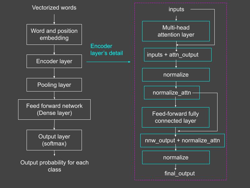
Figure 1: The overall transformer model (left). The encoder layer’s details are shown in the dashed pink box (right). Source: Mehreen Saeed
The Import Section
The first step is to import the following libraries into your code.
# Different layersfrom tensorflow.keras.layers import MultiHeadAttention, Input, Densefrom tensorflow.keras.layers import LayerNormalization, Layerfrom tensorflow.keras.layers import TextVectorization, Embedding, GlobalAveragePooling1D# For miscellaneous functionsfrom tensorflow.data import Datasetfrom tensorflow import convert_to_tensor, string, float32, shape, range, reshapefrom tensorflow.keras import utils# Keras modelsfrom tensorflow.keras import Model, Sequential# For datasetsfrom sklearn.datasets import fetch_20newsgroups# For evaluationfrom sklearn import metricsfrom sklearn.metrics import confusion_matrix, ConfusionMatrixDisplay# For math/arraysimport numpy as np# For plottingimport matplotlib.pyplot as pltLoad the Dataset
The scikit-learn library includes the 20-newsgroup dataset with an option to load the training or test data. The code below reads both train and test subsets using fetch_20newsgroups, converts the labels to categorical labels, and prints some statistics.
# Load the training dataset while removing headers, footers and quotestrain_dataset = fetch_20newsgroups(subset='train', random_state=0,remove=("headers", "footers", "quotes"))train_X, train_Y = (train_dataset.data, train_dataset.target)
# Test datasettest_dataset = fetch_20newsgroups(subset='test', random_state=0,remove=("headers", "footers", "quotes"))test_X, test_Y = (test_dataset.data, test_dataset.target)# Target classesnewsgroup_names = train_dataset.target_names# Total classesn_classes = len(train_dataset.target_names)# Convert to binary vectors to represent categoriestrain_Y_categorical = utils.to_categorical(train_Y)test_Y_categorical = utils.to_categorical(test_Y)
#Print statisticsprint("Total training sequences: ", len(train_X))print("Total test sequences: ", len(test_X))print("Target categories are: ", newsgroup_names)Total training sequences: 11314Total test sequences: 7532Target categories are: ['alt.atheism', 'comp.graphics', 'comp.os.ms-windows.misc', 'comp.sys.ibm.pc.hardware', 'comp.sys.mac.hardware', 'comp.windows.x', 'misc.forsale', 'rec.autos', 'rec.motorcycles', 'rec.sport.baseball', 'rec.sport.hockey', 'sci.crypt', 'sci.electronics', 'sci.med', 'sci.space', 'soc.religion.christian', 'talk.politics.guns', 'talk.politics.mideast', 'talk.politics.misc', 'talk.religion.misc']From the above output, we can see that the 20 categories overlap. For example, talk.politics.mideast and talk.politics.misc have many newsgroups in common. Strictly speaking, this is more of a multi-labeling task, where one newsgroup can be assigned to multiple classes. However, we’ll perform multi-class classification, where one example newsgroup is assigned to only one category.
An example newsgroup/data point is shown below. You can change the value of example_index to see more newsgroup texts and their categories.
example_index = 10print('Category: ', newsgroup_names[train_Y[example_index]])print('Corresponding text: ', train_X[example_index])
Category: sci.medCorresponding text:


There's been extensive discussion on the CompuServe Cancer Forum about Dr.Burzynski's treatment as a result of the decision of a forum member's fatherto undertake his treatment for brain glioblastoma. This disease isuniversally and usually rapidly fatal. After diagnosis in June 1992, thetumor was growing rapidly despite radiation and chemotherapy. The forummember checked extensively on Dr. Burzynki's track record for this disease.He spoke to a few patients in complete remission for a few years fromglioblastoma following this treatment and to an NCI oncologist who hadaudited other such case histories and found them valid and impressive.After the forum member's father began Dr. Burzynski's treatment inSeptember, all subsequent scans performed under the auspices of hisoncologist in Chicago have shown no tumor growth with possible signs ofshrinkage or necrosis.
The patient's oncologist, although telling him he would probably not livepast December 1992, was vehemently opposed to his trying Dr. Burzynski'streatment. Since the tumor stopped its rapid growth under Dr. Burzynski'streatment, she's since changed her attitude toward continuing thesetreatments, saying "if it ain't broke, don't fix it."
Dr. Burzynski is an M.D., Ph.D. with a research background who found aprotein that is at very low serum levels in cancer patients, synthesized it,and administers it to patients with certain cancer types. There is littleunderstanding of the actual mechanism of activity.Text Vectorization: Converting Words to Numbers
The training data we just read is a series of English sentences. We need to convert the textual data to numbers so that it can be input to the transformer model. One possible solution is to use the TextVectorization layer from the Keras library. This layer can be trained to learn a vocabulary consisting of all the unique words in a corpus using the adapt method. We can then use the trained vectorized layer to replace each word in a sentence with its corresponding dictionary index.
This small toy example should help you understand the working of this layer. Below we have two simple sentences that are converted to fixed-size numeric vectors of length 8. The learned dictionary and the corresponding vectorized sentences are printed at the end of the code. To help distinguish between different variables in this article, all the variable names related to the toy examples are preceded by “toy_”.
toy_sentences = [["I am happy today"], ["today weather is awesome"]]# Create the TextVectorization layertoy_vectorize_layer = TextVectorization(output_sequence_length=8,max_tokens=15)# Learn a dictionarytoy_vectorize_layer.adapt(Dataset.from_tensor_slices(toy_sentences))# Use the trained TextVectorization to replace each word by its# dictionary indextoy_vectorized_words = toy_vectorize_layer(convert_to_tensor(toy_sentences, dtype=string))print("Dictionary: ", toy_vectorize_layer.get_vocabulary())print("Vectorized words: ", toy_vectorized_words)Dictionary: ['', '[UNK]', 'today', 'weather', 'is', 'i', 'happy', 'awesome', 'am']Vectorized words: tf.Tensor([[5 8 6 2 0 0 0 0][2 3 4 7 0 0 0 0]], shape=(2, 8), dtype=int64)Vectorize the Training and Test Data
Let’s apply text vectorization to our training and test samples from the newsgroup dataset.
# The total distinct words to usevocab_size = 25000# Specify the maximum charancters to consider in each newsgroupsequence_length = 300
train_X_tensor = Dataset.from_tensor_slices(train_X)# TextVectorization layervectorize_layer = TextVectorization(output_sequence_length=sequence_length,max_tokens=vocab_size)# Adapt method trains the TextVectorization layer and# creates a dictionaryvectorize_layer.adapt(train_X_tensor)# Convert all newsgroups in train_X to vectorized tensorstrain_X_tensors = convert_to_tensor(train_X, dtype=string)train_X_vectorized = vectorize_layer(train_X_tensors)# Convert all newsgroups in test_X to vectorized tensorstest_X_tensors = convert_to_tensor(test_X, dtype=string)test_X_vectorized = vectorize_layer(test_X_tensors)
The Embedding Layer: Positional Encoding of Words and Indices
In all natural language processing tasks, the order of words within text is important. Changing the position of words in a sentence can change its entire meaning. The transformer model does not use any convolutions or recurrences, which is why we must explicitly add the positional information of words to the input data before the transformer processes it. The authors of “Attention Is All You Need” recommend using a sum of word embeddings and positional encodings as the input to the encoder. They also proposed their own scheme that uses sinusoids for mapping words and positions to the embedded vectors.
To keep things simple, instead of implementing embedding using sinusoids, we’ll use Keras’ Embedding layer, which initializes all embeddings to random numbers and later learns the embedding during the training phase. Here is an example on the smaller toy sentences to help you understand what the embedding layer does.
# Embedding for wordstoy_word_embedding_layer = Embedding(input_dim=15, output_dim=4)toy_embedded_words = toy_word_embedding_layer(toy_vectorized_words)# Embedding for positionstoy_position_embedding_layer = Embedding(input_dim=8, output_dim=4)toy_positions = range(start=0, limit=8, delta=1)toy_embedded_positions = toy_position_embedding_layer(toy_positions)The toy_embedded_words are the word embeddings corresponding to each sentence. Each word in a sentence is represented by a vector. As each vectorized toy sentence has a maximum length of eight, there are eight corresponding positions in a sentence. The embedded_toy_positions are the corresponding embeddings for the word positions. They are the same for all sentences. The two embeddings are summed together to form the output of the text preprocessing stage. Both word and position embeddings for this toy example are shown in Figure 2.
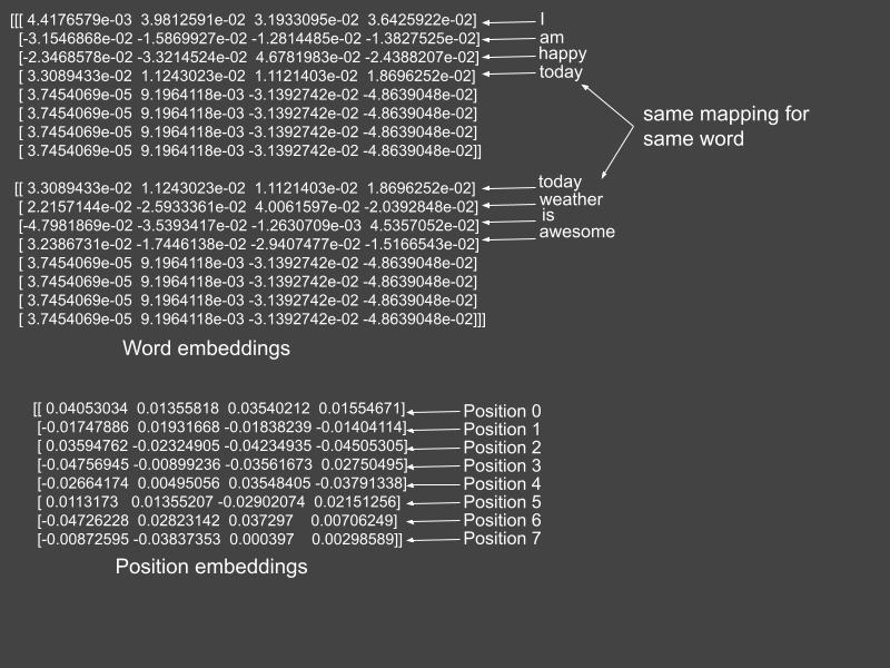
Figure 2: The word and position embeddings. The position embeddings are added to the word embeddings of each sentence. Source: Mehreen Saeed
Writing a Customized Embedding Layer
While the Keras’ Embedding layer implements the basic functionality for initializing and learning the encoding, there is no layer that adds the word and position embeddings to produce the final output. We have to write our own custom layer to implement this step. Below is our own EmbeddingLayer that has two Embedding layers:
- word_embedding: Maps words to their corresponding encodings
- position_embedding: Maps positions/word indices to their corresponding encoding
The call() method uses the Keras’ Embedding layer to compute the words, position embeddings, and return their sum.
class EmbeddingLayer(Layer):def __init__(self, sequence_length, vocab_size, embed_dim):super(EmbeddingLayer, self).__init__()self.word_embedding = Embedding(input_dim=vocab_size, output_dim=embed_dim)self.position_embedding = Embedding(input_dim=sequence_length, output_dim=embed_dim)
def call(self, tokens):sequence_length = shape(tokens)[-1]all_positions = range(start=0, limit=sequence_length, delta=1)positions_encoding = self.position_embedding(all_positions)words_encoding = self.word_embedding(tokens)return positions_encoding + words_encodingThe Encoder Layer
There is no direct implementation of the transformer encoder layer in Keras. However, we can write our own custom layer by making use of the MultiHeadAttention layer and the Dense layer.
The Multihead Attention Layer
In my tutorial on transformers, I explained the multihead layer in detail. The computations taking place in this layer appear in Figure 3.
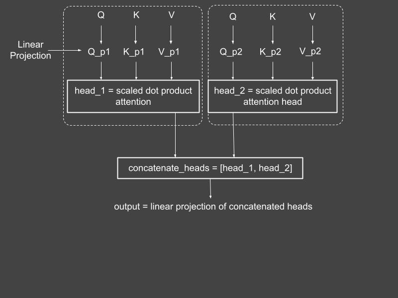
Figure 3: The multihead attention layer. Source: Mehreen Saeed
Fortunately, the Keras library includes an implementation of MultiHeadAttention layer. We’ll use this layer to build the encoder layer.
If you are interested in the nitty-gritty details of the Keras’ MultiHeadAttention layer, here is a toy example to help you understand. The MultiHeadAttention attention layer encapsulates a list of eight weights, which are:
- Index 0: Weights for linear projection of query
- Index 1: Bias corresponding to linear projection of query
- Index 2: Weights for linear projection of key
- Index 3: Bias corresponding to linear projection of key
- Index 4: Weights for linear projection of values
- Index 5: Bias corresponding to linear projection of values
- Index 6: Weights for linear projection of concatenated heads
- Index 7: Bias corresponding to linear projection of concatenated heads
toy_multihead = MultiHeadAttention(num_heads=1, key_dim=3)toy_x = np.array([[[1, 2, 3]]])toy_x_tensor = convert_to_tensor(toy_x, dtype=float32)toy_attn_output, toy_attn_wts = toy_multihead(toy_x_tensor, toy_x_tensor, return_attention_scores=True)print('Multihead layer output: \n', toy_attn_output)print('\nMultihead attention wts: \n', toy_attn_wts)print('\nTotal Layer weights: ', len(toy_multihead.get_weights()))Multihead layer output:tf.Tensor([[[ 2.0663598 1.4963739 -1.668928 ]]], shape=(1, 1, 3), dtype=float32)
Multihead attention wts:tf.Tensor([[[[1.]]]], shape=(1, 1, 1, 1), dtype=float32)
Total Layer weights: 8Implementing the Encoder Layer
The code implementing the custom EncoderLayer is shown below. The call() method implements the basic operations that take place in the encoder layer.
class EncoderLayer(Layer):def __init__(self, total_heads, total_dense_units, embed_dim):super(EncoderLayer, self).__init__()# Multihead attention layerself.multihead = MultiHeadAttention(num_heads=total_heads, key_dim=embed_dim)# Feed forward network layerself.nnw = Sequential([Dense(total_dense_units, activation="relu"),Dense(embed_dim)])# Normalizationself.normalize_layer = LayerNormalization()
def call(self, inputs):attn_output = self.multihead(inputs, inputs)normalize_attn = self.normalize_layer(inputs + attn_output)nnw_output = self.nnw(normalize_attn)final_output = self.normalize_layer(normalize_attn + nnw_output)return final_outputTo help you understand the computations taking place in the call() method, Figure 4 shows the encoder layer, along with the corresponding code that implements it.

Figure 4: The conceptual diagram of the encoder layer (at left) and the corresponding code (right). Source: Mehreen Saeed
Powering Up the Transformer
It’s time to construct our final transformer model from the EmbeddingLayer and EncoderLayer. We also need to add the GlobalAveragePooling1D layer, followed by a Dense layer. The final output of the transformer is produced by a softmax layer, where each unit of the layer corresponds to a category of the text documents.
The following code constructs a transformer model for supervised classification and prints its summary.
embed_dim = 64num_heads = 2total_dense_units = 60# Our two custom layersembedding_layer = EmbeddingLayer(sequence_length, vocab_size, embed_dim)encoder_layer = EncoderLayer(num_heads, total_dense_units, embed_dim)
# Start connecting the layers togetherinputs = Input(shape=(sequence_length, ))emb = embedding_layer(inputs)enc = encoder_layer(emb)pool = GlobalAveragePooling1D()(enc)d = Dense(total_dense_units, activation="relu")(pool)outputs = Dense(n_classes, activation="softmax")(d)
# Construct the transformer modeltransformer_model = Model(inputs=inputs, outputs=outputs)transformer_model.compile(optimizer="adam", loss="categorical_crossentropy", metrics=['accuracy', 'Precision', 'Recall'])transformer_model.summary()Model: "model"_________________________________________________________________Layer (type) Output Shape Param #=================================================================input_1 (InputLayer) [(None, 300)] 0_________________________________________________________________embedding_layer (EmbeddingLa (None, 300, 64) 1619200_________________________________________________________________encoder_layer (EncoderLayer) (None, 300, 64) 41148_________________________________________________________________global_average_pooling1d (Gl (None, 64) 0_________________________________________________________________dense_2 (Dense) (None, 60) 3900_________________________________________________________________dense_3 (Dense) (None, 20) 1220=================================================================Total params: 1,665,468Trainable params: 1,665,468Non-trainable params: 0_________________________________________________________________Training the Transformer
The code below trains the transformer model using a 33% split for the validation set.
history = transformer_model.fit(train_X_vectorized, train_Y_categorical, batch_size=32, epochs=4, validation_split=0.33)Epoch 1/4237/237 [==============================] - 49s 203ms/step - loss: 2.8578 - accuracy: 0.1054 - precision: 0.6364 - recall: 9.2348e-04 - val_loss: 2.2344 - val_accuracy: 0.2659 - val_precision: 0.7629 - val_recall: 0.0198Epoch 2/4237/237 [==============================] - 51s 215ms/step - loss: 1.4798 - accuracy: 0.5422 - precision: 0.8342 - recall: 0.3318 - val_loss: 1.3582 - val_accuracy: 0.6012 - val_precision: 0.7853 - val_recall: 0.4917Epoch 3/4237/237 [==============================] - 60s 252ms/step - loss: 0.6496 - accuracy: 0.7984 - precision: 0.9011 - recall: 0.7475 - val_loss: 1.2908 - val_accuracy: 0.6486 - val_precision: 0.7659 - val_recall: 0.5983Epoch 4/4237/237 [==============================] - 59s 250ms/step - loss: 0.3109 - accuracy: 0.9084 - precision: 0.9576 - recall: 0.8916 - val_loss: 1.4340 - val_accuracy: 0.6601 - val_precision: 0.7393 - val_recall: 0.6310The history object stores the learning history of our model. We have the following keys in the history.history object returned by the fit() method.
print(history.history.keys())dict_keys(['loss', 'accuracy', 'precision', 'recall', 'val_loss', 'val_accuracy', 'val_precision', 'val_recall'])The keys preceded by val_ indicate the metric corresponding to the validation set. The four metrics that are being recorded are:
- Loss: The categorical cross-entropy loss function
- Accuracy: Percentage of correctly classified examples
- Precision: Total true positives divided by the total instances labeled as positive. For multi-class classification, precision is computed for all classes and then averaged.
- Recall: Total true positives divided by the total number of examples that belong to the positive class. For multi-class classification, recall is calculated for all classes and then averaged.
Let’s visualize the learning history by plotting various metrics.
fig = plt.figure(figsize=(18,4))metric = ['loss', 'accuracy', 'precision', 'recall']validation_metric = ['val_loss', 'val_accuracy', 'val_precision', 'val_recall']
for i,j,k in zip(metric, validation_metric, np.arange(len(metric))):fig.add_subplot(141+k)
plt.plot(history.history[i])plt.plot(history.history[j])plt.legend(['Training', 'Validation'])plt.title('Training and validation ' + i)plt.xlabel('Epoch Number')plt.ylabel('Accuracy')
plt.show()---------------------------------------------------------------------------
NameError Traceback (most recent call last)
<ipython-input-1-9278e0ea23a1> in <module>()----> 1 fig = plt.figure(figsize=(18,4))2 metric = ['loss', 'accuracy', 'precision', 'recall']3 validation_metric = ['val_loss', 'val_accuracy', 'val_precision', 'val_recall']45 for i,j,k in zip(metric, validation_metric, np.arange(len(metric))):

NameError: name 'plt' is not definedViewing the Learned Word and Position Embeddings
Keras’ Embedding layer starts with random encodings and learns them during the training phase. You can visualize these embeddings by rendering them as an image.
The code below creates two models, i.e., a random_embeddings_model that uses an initialized untrained embedding layer and a learned_embeddings_model that is built from the learned embedding layer of our transformer model. Once the models are created, the first training example is passed through both models and its output is rendered as an image. A comparison of both renderings show how the embeddings start with completely random values, which take on a more smooth and ordered form after training. This learned embeddings layer, therefore, assigns each newsgroup example a unique signature that distinguishes it from from other newsgroups.
# Get the random embeddingsrandom_embedding_layer = EmbeddingLayer(sequence_length, vocab_size, embed_dim)random_emb = random_embedding_layer(inputs)random_embeddings_model = Model(inputs=inputs, outputs=random_emb)random_embedding = random_embeddings_model.predict(train_X_vectorized[0:1,])random_matrix = reshape(random_embedding[0, :, :], (sequence_length, embed_dim))
# Get the learned embeddingslearned_embeddings_model = Model(inputs=inputs, outputs=emb)learned_embedding = learned_embeddings_model.predict(train_X_vectorized[0:1,])learned_matrix = reshape(learned_embedding[0, :, :], (sequence_length, embed_dim))
# Render random embeddingsfig = plt.figure(figsize=(15, 8))ax = plt.subplot(1, 2, 1)cax = ax.matshow(random_matrix)plt.gcf().colorbar(cax)plt.title('Random embeddings', y=1)
# Render learned embeddingsax = plt.subplot(1, 2, 2)cax = ax.matshow(learned_matrix)plt.gcf().colorbar(cax)plt.title('Learned embeddings', y=1)plt.show()
Evaluating the Transformer’s Classification Performance
We can evaluate our trained model on the test set using different methods, discussed below.
The Accuracy, Precision, and Recall Metrics
The accuracy, precision, and recall metrics were all recorded during training. The evaluate() method of the transformer_model object returns these metrics in an array. Let’s print them for both the training and test sets.
train_metrics = transformer_model.evaluate(train_X_vectorized, train_Y_categorical)test_metrics = transformer_model.evaluate(test_X_vectorized, test_Y_categorical)print('Training set evaluation - Accuracy:\n', train_metrics[1],' Precision: ', train_metrics[2], ' Recall: ', train_metrics[3])print('Test set evaluation - Accuracy:\n', test_metrics[1],' Precision: ', test_metrics[2], ' Recall: ', test_metrics[3], '\n')354/354 [==============================] - 24s 67ms/step - loss: 0.6031 - accuracy: 0.8531 - precision: 0.9115 - recall: 0.8366236/236 [==============================] - 17s 71ms/step - loss: 1.7248 - accuracy: 0.6053 - precision: 0.6846 - recall: 0.5746Training set evaluation - Accuracy: 0.8531023263931274 Precision: 0.911498486995697 Recall: 0.836574137210846Test set evaluation - Accuracy: 0.6052840948104858 Precision: 0.6845934987068176 Recall: 0.5746150016784668The Confusion Matrix
The code below computes the confusion matrix and displays it using the functions provided in the scikit-learn library.
# For confusion matrixtest_predict = transformer_model.predict(test_X_vectorized)test_predict_labels = np.argmax(test_predict, axis=1)
fig, ax = plt.subplots(figsize=(15, 15))
# Create and display the confusion matrixtest_confusion_matrix = confusion_matrix(test_Y, test_predict_labels)cm = ConfusionMatrixDisplay(confusion_matrix=test_confusion_matrix,display_labels=newsgroup_names)cm.plot(xticks_rotation="vertical", ax=ax)plt.title('Confusion Matrix of the Test Set')plt.show()print('Correct classification: ', np.sum(np.diagonal(test_confusion_matrix)), '/', len(test_predict_labels))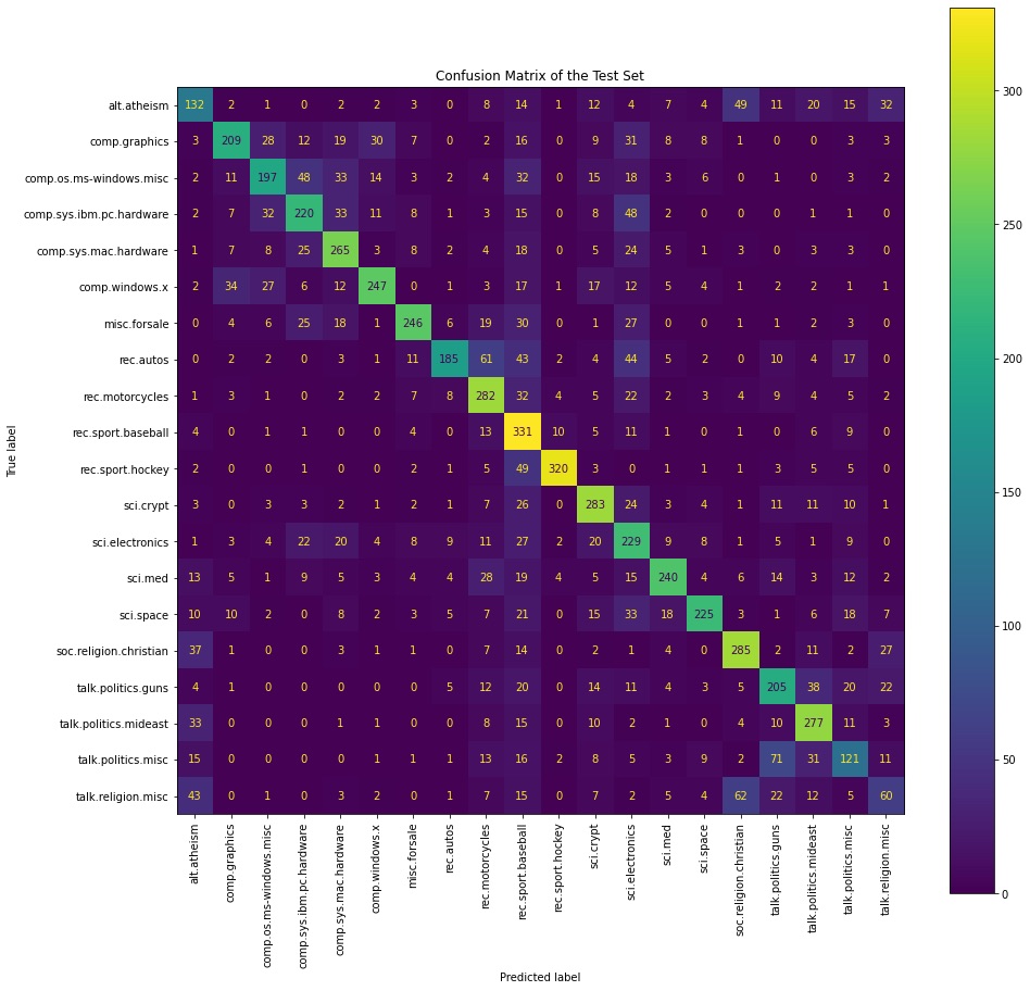
Correct classification: 4559 / 7532At a first glance, the various scores on the test set don’t look very good. However, we can understand the results by looking at the confusion matrix and observing where the errors are taking place. Because many categories/topics in the newsgroup dataset are similar and can contain overlapping content, a newsgroup can belong to multiple classes at the same time. We can see from the confusion matrix that a majority of errors have occurred in similar classes. For example, when the true label is comp.windows.x, many examples are classified into comp.graphics or comp.os.ms-windows.misc. This is also the case for sci.religion.christian and talk.religion.misc.
Next Steps
Now you know how to develop a simple transformer model for solving supervised classification problems. The encoder layer is the basic ingredient required for classification tasks, and you can now easily add a decoder layer to this model and experiment with sequence-to-sequence tasks such as language translation, sentence paraphrasing, and even document summarization.
You can also add more encoder layers to the transformer model we just built and experiment with different values of sequence lengths, embedding dimensions, and number of dense units in the feed forward layer. The concept of self-attention, along with its implementation in transformers, creates a powerful model that is already being used to solve many real-world problems. Transformers are likely to make their way into more and more machine learning tasks in the near future.
You can run the entire code shown in this tutorial in Google Colab or download the Python notebook here. This is the final installment in our series on using TensorFlow for supervised classification tasks.
Learn More
- Using TensorFlow for Supervised Classification Tasks: How to Build an Autoencoder
Popular
Dive in
Related
Blog
How to Build a Faster Vision Transformer for Supervised Image Classification
By Mehreen Saeed • Sep 21st, 2022 • Views 9K
Video
How to Build an Effective AI Strategy for Business
By Catherine Williams • Oct 6th, 2021 • Views 4.5K
Blog
How to Build a Faster Vision Transformer for Supervised Image Classification
By Mehreen Saeed • Sep 21st, 2022 • Views 9K
Video
How to Build an Effective AI Strategy for Business
By Catherine Williams • Oct 6th, 2021 • Views 4.5K