In their seminal paper “Attention Is All You Need,” Ashish Vaswani and colleagues proposed the transformer architecture solely based on the attention mechanism. Engineers have successfully applied this model to implement many natural language processing tasks. Later in 2021, Alexey Dosovitskiy and his co-authors showed how to modify the transformer architecture to solve problems in the computer vision domain. The only addition to the pure transformer is an added layer that breaks up an image into smaller image patches that act like tokens.

The resulting model, called a “vision transformer” (ViT), works well for image data. However, the training phase of ViTs involves many operations and can be pretty slow. Michael Ryoo and his colleagues showed one possible method of speeding up the computations of the training stage by adding a token learning layer called TokenLearner to the network.

In an earlier tutorial, I showed how to build a transformer for supervised classification of text documents. This time, I’ll modify this model to build a ViT and use it to classify images. As a second step, I’ll show you how to add a token learning layer to the transformer model to create a faster ViT model.

My goal is to show you how the ViT works and how the token learner improves its performance. I’ll keep everything simple; you won’t see any fancy preprocessing or sophisticated fine-tuning of the model to beat the accuracy of existing systems.

Prerequisites

Before we get started, be aware that you’ll need some background knowledge to understand this tutorial. If you are at a beginning stage, I suggest you first read through these articles, in sequence:

1. Attention Models: What They Are and Why They Matter
2. Transformers: What They Are and Why They Matter
3. How to Build a Transformer for Supervised Classification Using Keras and TensorFlow

The Overall ViT Architecture

The ViT you are about to build has the structure shown in Figure 1. After tokenizing the image, the transformer passes the token images through an embedding layer, followed by four encoder layers. The output from the last encoder layer is input to a global average pooling layer and then passed through a feedforward neural network.

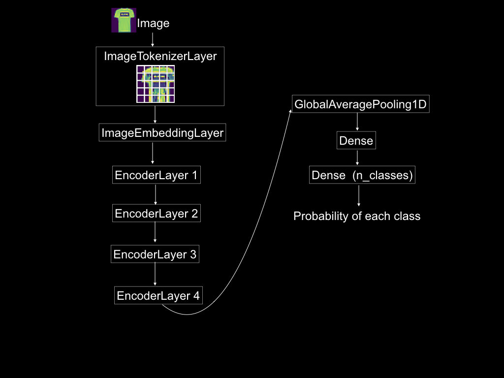
Figure 1: The vision transformer architecture. Source: Mehreen Saeed

The Import Section

As a first step, import the following libraries:

Load the Dataset

We’ll use the Fashion-MNIST dataset, which consists of 28-by-28 grayscale images of different fashion items. In the code below, I have set n_classes to four so that you can run this code quickly on four classes. Change this value to 10 to run the example on the entire dataset.

The following code reads the dataset and prints some statistics.

As these images are grayscale, but you can reshape them to a 3D array with one color channel. This way, this code will work for RGB images as well.

The Image Tokenizer Layer

For image data, the key is to understand what a token represents. One possibility is to let each pixel represent a token. However, this would not scale well with large image datasets. In the ViT architecture, Dosovitskiy and his colleagues used equal-sized patches of images to act as tokens. This sequence of tokens is then input to a traditional transformer with a minimal change to its architecture.

Fortunately, the TensorFlow library includes an extract_patches() method to break an image into smaller patches of fixed size. You can use this function to implement your own layer for tokenizing an image. In the code below, ImageTokenizerLayer is a custom class for tokenizing images. The call() method of this class creates the image patches and returns them.

Because the tokenization step is needed only once, you can store the tokens corresponding to the training set and use them as input to the ViT. In the code below, the dimensions of each token are the square root of the dimensions of the training and test images. However, you can change the patch size to a different value also. The two variables train_tokens and test_tokens store fixed-size tokens of each image. The tokens are also rendered below.

A few things to note:

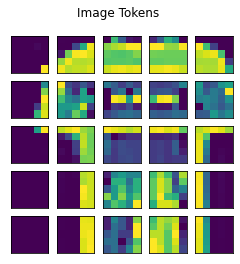
1. A single input image has 28 by 28 dimensions.
2. The input image is broken into 25 tokens of size 5 by 5.
3. Each 5-by-5 image token/patch is vectorized into a 1D array of size 25.
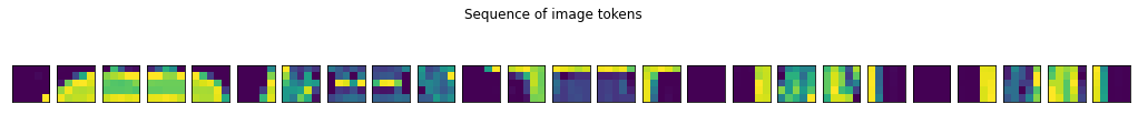
4. In the tokenized training dataset, each image is split into a sequence of tokens. One image has 5-by-5-by-25 dimensional representation.
5. n_rows and n_cols represent the total image tokens along the rows and columns, respectively. The total number of image tokens is, therefore, n_rows * n_cols.

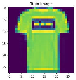
Writing a Customized Embedding Layer for the ViT

In a pure transformer architecture, all word tokens are encoded by summing their embeddings and their encoded positions. In the case of a ViT, the embedding layer projects an image linearly and sums it with its corresponding positional encoding. In this way, the positional encoding helps retain the order of a token in the sequence.

Below, you can see the implementation of a custom layer for encoding each image token. The call() method implements the following steps:

1. Normalize the input image tokens.
2. Project the normalized image tokens by using a Dense layer.
3. Encode the positions using TensorFlow Embedding layer.
4. Add the projections and the encoded positions. Return their sum.

Here, the length of the resulting embedding is stored in the variable embed_dim, whose value can be set by a user. Hence, the embedding layer produces an output of size total_tokens x embed_dim. Again, keep in mind that total_tokens = n_rows * ncols.

The Encoder Layer

In “How to Build a Transformer for Supervised Classification,” I showed you how to build a single encoder layer by sub-classing the Layer class. We’ll use the same implementation for the ViT. Just to recall, the encoder layer implements multihead attention followed by a feedforward network and a normalization layer.

Build the ViT

It’s time to construct the final ViT model from the ImageEmbeddingLayer and EncoderLayer. The final output of the transformer is produced by a softmax layer, where each unit of the layer corresponds to a category of the input image.

The code below constructs a ViT with four encoder layers followed by GlobalAveragePooling1D layer, an intermediate Dense layer, and the output Dense layer (refer to Figure 1).

Let’s look at the model summary.

Training the ViT

The code below trains the transformer model using a 33% split for the validation set.

View the Learning History

The history object stores the learning history of our model. The fit() method returns the following keys in the history.history object.

Let’s visualize the learning history by plotting various metrics.

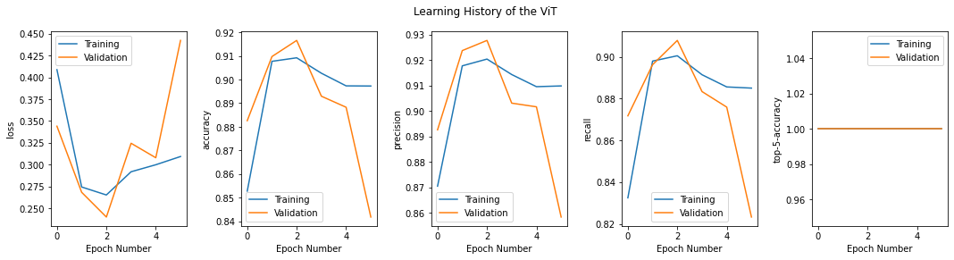
Evaluating the ViT’s Classification Performance

The evaluate() method returns all the metrics that you specified during the training stage.

How To Make the ViT Faster

While there are several methods for making the ViT faster, we’ll implement the TokenLearner of Ryoo and colleagues. The TokenLearner layer learns to identify important tokens in the input data. It then dynamically selects these tokens conditioned on the input, reducing the number of tokens used for classifying images. This algorithm mimics the element-wise spatial self-attention.

What is the Basic TokenLearner Algorithm?

Here is the basic algorithm for the layer that implements the TokenLearner. In the algorithm below, n_maps represents the number of feature maps and is a user-supplied parameter.

1. Compute weight maps conditioned on the inputs. The number of weight maps are n_maps. They effectively represent the attention weights. The weights have dimensions n_rows x n_cols x n_maps.
2. Reshape the weights to total_tokens x n_maps.
3. Multiply the weight maps by the inputs to get weighted inputs. The input size is total_tokens x embed_dim and the resulting weighted input size is total_tokens x n_maps x embed_dim.
4. Apply spatial global average pooling to reduce the dimensions of the weighted inputs to n_maps x embed_dim.

Figure 2 shows all these computations on the left.

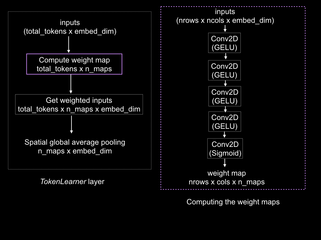
Figure 2: The token learning layer. Source: Mehreen Saeed

How Is the Weight Map Computed?

Ryoo and colleagues compute the weight map of the TokenLearner as follows:

1. Reshape the inputs to n_rows x n_cols x embed_dim.
2. Pass the inputs through a series of convolution layers with a Gaussian Error Linear Unit (GELU) activation function.
3. Pass the convolved output through a convolution layer with sigmoid activation function. The dimensions of the result are n_rows x n_cols x n_maps.

The processing is shown on the right in Figure 2.

Where Is the Token Learner in the Transformer Network?

Ryoo and colleagues suggest you place the TokenLearner layer anywhere between the transformer encoder layers. They experimented with placing this layer at different points in the network. They observed that inserting the TokenLearner after the initial one quarter of the network reduces the computations to less than a third of the baseline with no compromise in accuracy. Moreover, if this layer is inserted further down in the network, the resulting model has improved accuracy.

Below is the code for the custom TokenLearningLayer. The fast_vit transformer model places the TokenLearningLayer after the two encoder layers, as shown in the figure below.

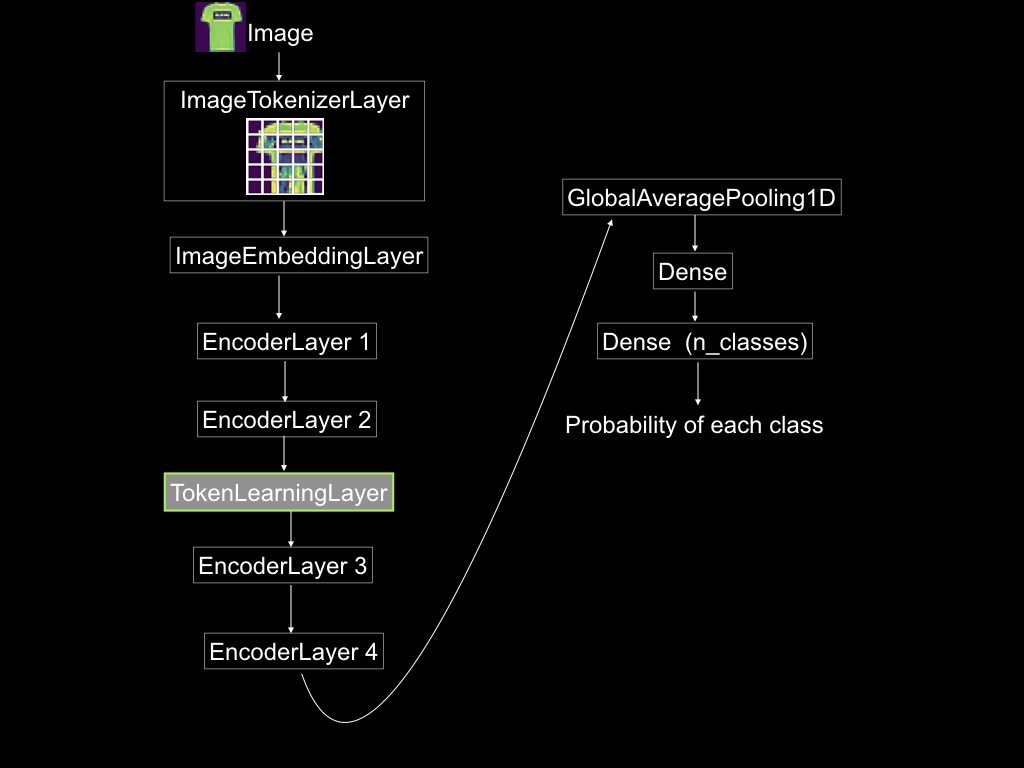
Figure 3: The overall ViT architecture with a token learning layer. Source: Mehreen Saeed

After creating the TokenLearningLayer, you can build the transformer with this layer after two encoder layers.

Next, let’s look at the summary of the model.

The summary of fast_vit model shows that the token_learning_layer takes a 25-by-128 input and reduces it to a 4-by-128 output. Hence, the subsequent encoder layers process 4-by-128 inputs—that is, four tokens instead of 25, thereby reducing the overall number of computations for training the ViT.

We can view the learning history of the fast ViT model.

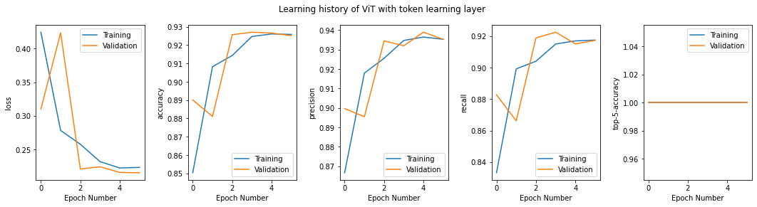
train_metrics_fast = fast_vit.evaluate(train_tokens, train_Y_categorical)

What Do the Results Indicate?

Adding a TokenLearningLayer to the network reduces the number of parameters of the layers following it, which also reduces the training time. In this example, I have used the time class to estimate the CPU time for training both the ViT and the fast ViT models. The overall time and the ms/step are both less for the later model. While this may be a crude method to judge the running time of a function, it still gives us a pretty good idea of the reduction in overall computation time. You can use more sophisticated measures for profiling.

Also, if you run this multiple times, you’ll note that the accuracy of both models is about the same, if not better, for the fast ViT model in terms of the metrics.

For larger datasets with bigger images, you may have deeper networks. In this case, you would see a significant reduction in the number of variables involved and computation time.

What’s Next?

Now that you know how to build a TokenLearner layer, you can experiment with different transformer hyper-parameters including the number of encoder layers, number of heads used in the encoder layer, number of feature maps in the TokenLearner and the number of dense units. For larger datasets, you may want to add parameters to stabilize weight training during the training phase. If you want to add the TokenLearner again to the transformer, you’ll have to use it with a TokenFuser, which remaps the feature maps back to their original spatial dimension.

Learn More

1. An Image Is Worth 16X16 Words: Transformer for Image Recognition at Scale
2. TokenLearner: Adaptive Space-Time Tokenization for Videos
3. Attention Models: What They Are and Why They Matter
4. Transformers: What They Are and Why They Matter
5. How to Build a Transformer for Supervised Classification