Articles
June 2, 2022
How to Build an Autoencoder Using TensorFlow
# TensorFlow
# Autoencoder
Here's how to build an autoencoder for image compression, image reconstruction, and supervised learning using the TensorFlow library.

Mehreen Saeed
In this article, I'll discuss using TensorFlow for supervised classification tasks, and we’ll work with a dataset of faces to build a simple autoencoder. We’ll use it for reconstructing the original face images and also visualize the latent space and build a supervised classifier from it that performs face recognition. For the implementation part, we’ll use TensorFlow and Keras library to build our model.
An autoencoder has two parts: an encoder and a decoder. The encoder learns a latent representation of the input data, and the decoder is trained to reconstruct the original inputs from the latent representations. The autoencoder has the following applications.
- It autoencoder approximates the original input points from the latent representations. This makes it useful for data recovery from corrupt inputs.
- As the autoencoder learns a latent representation of the input data, it can be designed so that the dimensions of this latent space is much smaller than the original input dimensions. Hence, an autoencoder can be used for data compression.
- Autoencoders find their application for data augmentation. The outputs from the autoencoder represent synthetic data and, hence, can be added to the original training set to increase its size.
- You can use the latent representation from an autoencoder to learn classification and regression tasks.
Here's how to get started building your own autoencoder. (Note: You can run the code shown in this tutorial in Google Colab or download the Python notebook here. Output shown from the code examples this article will not match the output that you get at your end: The output will vary with each run of the program because of the stochastic (random) nature of the algorithms involved.)
A Conceptual Diagram of the Autoencoder
Figure 1 below shows a conceptual diagram of the autoencoder we are about to build. The encoder appears in green, the decoder in pink. The input to the encoder is an rxc face image. The encoder uses the Flatten layer to vectorize the image to an r*c dimensional vector. The flatten layer passes the input to a dense layer, where the dense layer has half as many units as the original image pixels. The final layer of the encoder is the Dense layer with m units, where m is much smaller than the number of input image pixels. This is the latent representation of the input. Effectively, the encoder compresses the input to a smaller representation.
The decoder expands the encoder’s latent representation to produce an approximation of the input image. Hence, in this block, a smaller dense layer is followed by a bigger dense layer.
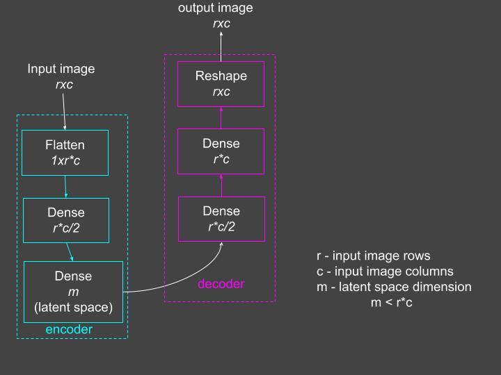
Figure 1: The autoencoder model. Flatten and reshape layers reshape the received inputs without changing the values. Source: Mehreen Saeed
The Import Section
Before starting the implementation, import the following libraries/modules in your code.
from tensorflow.keras import Sequentialfrom tensorflow.keras.models import Modelfrom tensorflow.keras.layers import Input, Densefrom tensorflow.keras.layers import Reshape, Flatten# For datasetfrom sklearn.datasets import fetch_lfw_peoplefrom sklearn.model_selection import train_test_split# For miscellaneous functionsfrom tensorflow.keras import utils# For array functionsimport numpy as np# For plottingimport matplotlib.pyplot as plt# For confusion matrixfrom sklearn.metrics import confusion_matrix, ConfusionMatrixDisplayLoad the ‘Labeled Faces in the Wild’ People Dataset
The scikit-learn library includes the Labeled Faces in the Wild (LFW) dataset, which consists of gray scale face images of different people. Because the dataset is imbalanced, we’ll load only the face images of people with at least 100 images included. We’ll also resize each image to half its dimensions to make the dataset more manageable.
Let’s load the dataset and display a few images along with some data statistics.
# Read the datalfw_people = fetch_lfw_people(min_faces_per_person=100, resize=0.5)# Get statistics of datan_samples, r, c = lfw_people.images.shapetarget_names = lfw_people.target_namesn_classes = target_names.shape[0]
# Display first 8 images of datasettotal_cols = 8fig, ax = plt.subplots(nrows=1, ncols=total_cols,                      figsize=(18,4),                      subplot_kw=dict(xticks=[], yticks=[]))
for j in range(total_cols):    ax[j].imshow(lfw_people.images[j, :, :])plt.title('First 8 Dataset Images', y=-0.2, x=-4)    plt.show()
# Print statisticsprint('STATISTICS')print('Dataset has ', n_samples, 'sample images')print('Each image is ', r, 'x', c)print('Faces are of:\n', target_names)
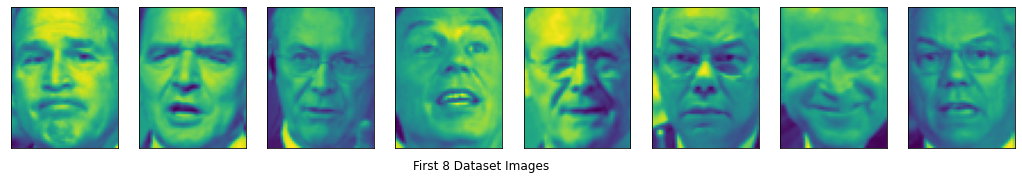
STATISTICSDataset has 1140 sample imagesEach image is 62 x 47Faces are of: ['Colin Powell' 'Donald Rumsfeld' 'George W Bush' 'Gerhard Schroeder' 'Tony Blair']Prepare the Train and Test Data
The next step is to prepare the train and test data. The code below implements the following steps:
- Use train_test_split() method to split the dataset into a 75% training and 25% test set.
- Normalize each image’s pixel values to lie between 0 and 1. Because the grayscale images have pixel values between 0 and 255, we can divide each pixel value by 255 to normalize the entire image.
- Use the to_categorical() method to convert each target value (range [0, 5]) to a five dimensional binary categorical vector.
- Print the training and test data statistics.
X = lfw_people.imagesy = lfw_people.target# Create train and test setstrain_X, test_X, train_Y, test_Y = train_test_split( X, y, test_size=0.25, random_state=0)# Normalize each imagetrain_X = train_X/255test_X = test_X/255# Create 5 dimensional binary indicator vectorstrain_Y_categorical = utils.to_categorical(train_Y)test_Y_categorical = utils.to_categorical(test_Y)# Print statisticsprint("Training data shape: ", train_X.shape)print("Training categorical labels shape: ", train_Y_categorical.shape)print("Test data shape: ", test_X.shape)print("Test categorical labels shape: ", test_Y_categorical.shape)Training data shape: (855, 62, 47)Training categorical labels shape: (855, 5)Test data shape: (285, 62, 47)Test categorical labels shape: (285, 5)Create the Autoencoder Model
The code below shows how you can use the Flatten, Dense and Reshape layers to create the autoencoder model shown in Figure 2. The value of the latent_dimension is set at 420. You can experiment with different values of this variable.
Because we want the input images to match the output images, we optimize with respect to the mean square error (mse). This can be specified as a parameter to the compile() method.
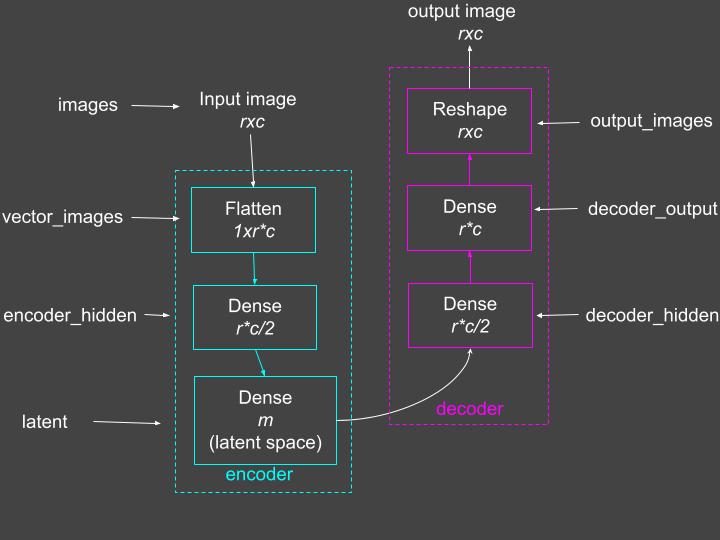
Figure 2: The autoencoder model with layer names used in the code. Source: Mehreen Saeed
latent_dimension = 420input_shape = (train_X.shape[1], train_X.shape[2])n_inputs = input_shape[0]*input_shape[1]images = Input(shape=(input_shape[0], input_shape[1], ))vector_images = Flatten()(images)# encoder encoder_hidden = Dense(n_inputs/2, activation='relu')(vector_images)latent = Dense(latent_dimension, activation='relu')(encoder_hidden)# define decoderdecoder_hidden = Dense(n_inputs/2, activation='relu')(latent)# output dense layerdecoder_output = Dense(n_inputs, activation='linear')(decoder_hidden)output_images = Reshape((input_shape[0], input_shape[1], ))(decoder_output)# define autoencoder modelautoencoder = Model(inputs=images, outputs=output_images)# compile autoencoder modelautoencoder.compile(optimizer='adam', loss='mse')Now let’s look at the summary of the autoencoder model we just built.
autoencoder.summary()Model: "model"_________________________________________________________________Layer (type) Output Shape Param # =================================================================input_1 (InputLayer) [(None, 62, 47)] 0 _________________________________________________________________flatten (Flatten) (None, 2914) 0 _________________________________________________________________dense (Dense) (None, 1457) 4247155 _________________________________________________________________dense_1 (Dense) (None, 420) 612360 _________________________________________________________________dense_2 (Dense) (None, 1457) 613397 _________________________________________________________________dense_3 (Dense) (None, 2914) 4248612 _________________________________________________________________reshape (Reshape) (None, 62, 47) 0 =================================================================Total params: 9,721,524Trainable params: 9,721,524Non-trainable params: 0_________________________________________________________________Training the Autoencoder
Now we are ready to train the autoencoder model. The fit() method below trains the model and returns a history object with details of the entire training process.
# fit the autoencoder model to reconstruct inputhistory = autoencoder.fit(train_X, train_X, epochs=100, validation_split=0.33, verbose=0)We can visualize the entire learning process by using the values stored in the dictionary object of history. The following code prints the keys of the history.history dictionary object and plots the training and validation loss for each epoch. As expected, the value of the loss function for the training set is lower than the loss value for the validation set.
print('Keys of history.history: ', history.history.keys())
fig = plt.figure(figsize=(15,4))plt.plot(history.history['loss'])plt.plot(history.history['val_loss'])plt.legend(['Training loss', 'Validation loss'])plt.title('Training and Validation Loss')plt.xlabel('Epoch Number')plt.ylabel('Loss')plt.show()Keys of history.history:  dict_keys(['loss', 'val_loss'])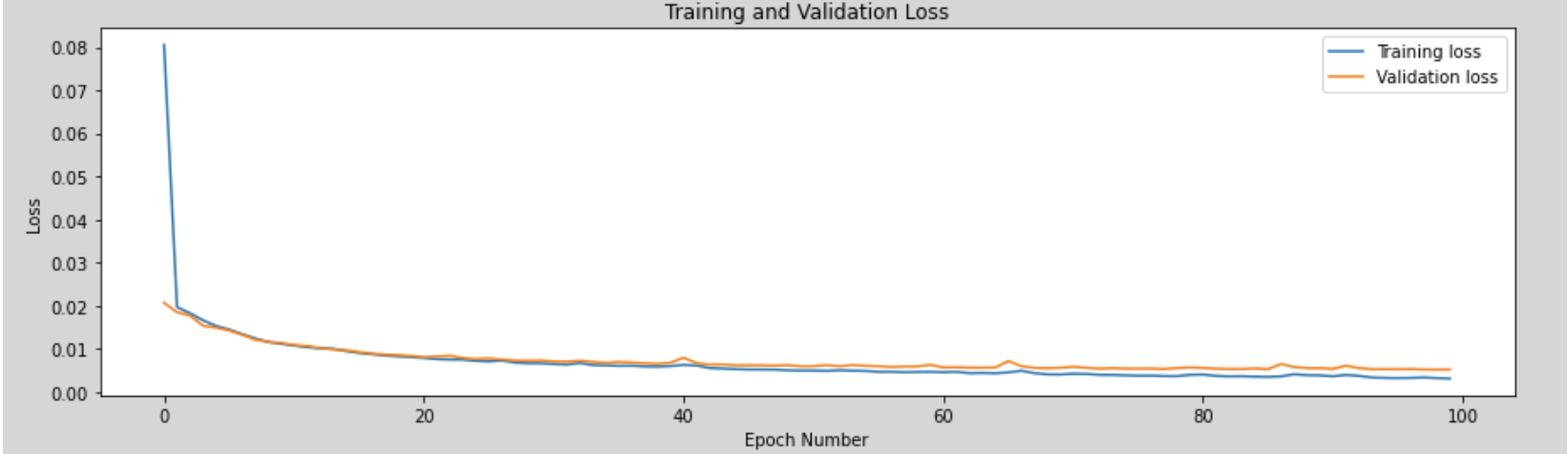
Reconstructing the Input Images
After training the autoencoder, we can look at what the reconstructed input images look like. The predict() method returns the output of the autoencoder for the inputs specified as a parameter. The code below displays the first eight images of the test set in the first row and their corresponding reconstructions in the second row.
# Reconstructionreconstructed_test = autoencoder.predict(test_X)# Display the inputs and reconstructionstotal_cols = 8fig, ax = plt.subplots(nrows=2, ncols=total_cols,                      figsize=(18,4),                      subplot_kw=dict(xticks=[], yticks=[]))
for j in range(total_cols): ax[0, j].imshow(test_X[j, :, :]) ax[1, j].imshow(reconstructed_test[j, :, :])plt.title('Input Images (Top Row) and Their Reconstruction by the Autoencoder (Bottom Row)', y=-0.4, x=-5) plt.show() 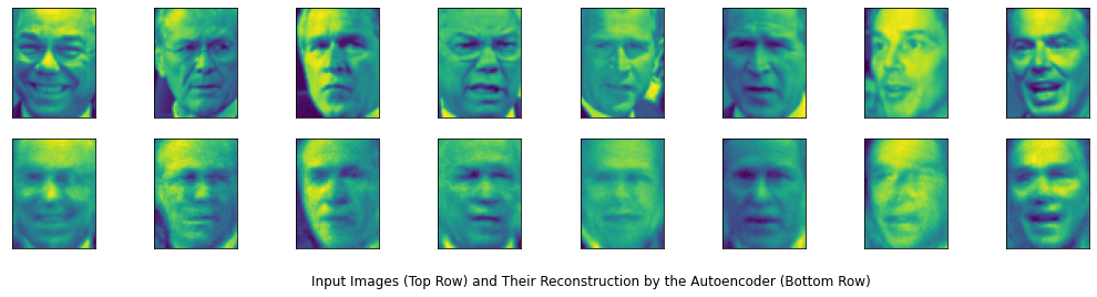
The reconstructed images are quite interesting. We can see that they are an approximation of the original images and each closely replicates the facial expression of the input face. This makes them useful for augmenting a limited training set with more examples. You can generate as many images as needed by training the autoencoder multiple times. The reconstructed faces will vary with each run as the weights of the autoencoder are initialized randomly.
Dissecting the Encoder
TensorFlow allows you to access the different layers of a model. You can easily retrieve the encoder block of the autoencoder by using the Model() method and instantiating it with the input images and output latent layer we created earlier. Let’s look at the summary of the encoder model.
# Encoder modelencoder_model = Model(inputs=images, outputs=latent)encoder_model.summary()Model: "model_1"_________________________________________________________________Layer (type) Output Shape Param # =================================================================input_1 (InputLayer) [(None, 62, 47)] 0 _________________________________________________________________flatten (Flatten) (None, 2914) 0 _________________________________________________________________dense (Dense) (None, 1457) 4247155 _________________________________________________________________dense_1 (Dense) (None, 420) 612360 =================================================================Total params: 4,859,515Trainable params: 4,859,515Non-trainable params: 0_________________________________________________________________The summary shows that we started out with an input of 2,914 (62x47) pixels and reduced it to only 420 outputs. These 420 outputs are an internal/latent space representation of the corresponding input image. The output of the encoder is hard for us to interpret. However, we can give it a try and visualize it by displaying it as an image. The code below arbitrarily reshapes the latent representation to a 20x21 image and renders it. The top row shows the input training image, and the bottom row shows the corresponding latent representation.
# Encoder outputencoder_output = encoder_model.predict(train_X)
latent_dim = encoder_output.shape[1]latent_shape = (20,21)# Plot the first 8 images and their corresponding latent representationtotal_cols = 8fig, ax = plt.subplots(nrows=2, ncols=total_cols,                      figsize=(18,4),                      subplot_kw=dict(xticks=[], yticks=[]))
for j in range(total_cols): train_image = train_X[j, :, :] ax[0, j].imshow(train_image) encoder_image = np.reshape(encoder_output[j, :], latent_shape) ax[1, j].imshow(encoder_image)plt.title('Input Images (Top Row) and Their Encoder Latent Representation (Bottom Row)', y=-0.4, x=-4) plt.show() 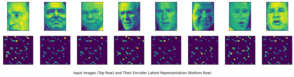
Using the Autoencoder for Supervised Learning
Strictly speaking, an autoencoder is not a supervised learning model, since it is trained with unlabeled images. However, we can use its latent representation to train a supervised learning model. The code below instantiates a classifier model by using all the layers of the autoencoder, from the vector_images layer up to the decoder_hidden layer. It then appends the model with a softmax layer that contains as many units as the number of classes/categories present in our dataset.
In the classifier model, we’ll set all the encoder layers to be nontrainable. This way the input image will be converted to its learned latent representation to be further processed by the classifier. The classifier will start training with the decoder weights tuned by the autoencoder and fine-tune them further to learn the classification of each latent representation. Figure 3 shows a block diagram of the classifier created from the autoencoder model. Now that we have a multiclass classification problem, we can use the ‘categorical_crossentropy’ as our loss function when compiling the model.
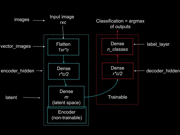
Figure 3: The classifier model created from the encoder. Source: Mehreen Saeed
# Create classifier modelclassifier = Sequential()label_layer = Dense(n_classes, activation='softmax')(decoder_hidden)classifier = Model(inputs=images, outputs=label_layer)
# Set the encoder layers to non-trainablefor layer in classifier.layers[:-2]:    layer.trainable=False
# Compile the model classifier.compile(optimizer='adam', loss='categorical_crossentropy', metrics=['accuracy'])Here is the summary of the classifier model. It has 620,687 trainable parameters associated with the last two layers. The rest of the weights up through the encoder layer are nontrainable.
classifier.summary()Model: "model_2"_________________________________________________________________Layer (type) Output Shape Param # =================================================================input_1 (InputLayer) [(None, 62, 47)] 0 _________________________________________________________________flatten (Flatten) (None, 2914) 0 _________________________________________________________________dense (Dense) (None, 1457) 4247155 _________________________________________________________________dense_1 (Dense) (None, 420) 612360 _________________________________________________________________dense_2 (Dense) (None, 1457) 613397 _________________________________________________________________dense_4 (Dense) (None, 5) 7290 =================================================================Total params: 5,480,202Trainable params: 620,687Non-trainable params: 4,859,515_________________________________________________________________Let’s train the classifier using the fit() method.
history = classifier.fit(train_X, train_Y_categorical, epochs=150, validation_split=0.33, verbose=0)Evaluate the Classifier
The code below prints the classification accuracy on the training and test sets. Because this is a multiclass classification problem, it’s good to observe the confusion matrix. TensorFlow’s math module provides a routine for computing the confusion matrix, but we’ll use the method provided by the scikit-learn library. This library also includes a nice method for displaying the confusion matrix with fancy colors. Now you have reasonably good accuracy on the face classification task without doing any preprocessing, hyper-parameter tuning, and model selection.
train_loss, train_acc = classifier.evaluate(train_X,  train_Y_categorical)test_loss, test_acc = classifier.evaluate(test_X,  test_Y_categorical)print('Classification accuracy on training set: ', train_acc)print('Classification accuracy on test set: ', test_acc)27/27 [==============================] - 0s 6ms/step - loss: 0.2781 - accuracy: 0.93689/9 [==============================] - 0s 6ms/step - loss: 0.5743 - accuracy: 0.8596Classification accuracy on training set:  0.9368420839309692Classification accuracy on test set:  0.859649121761322# Get the classifier outputstest_predict = classifier.predict(test_X)# Get the classification labelstest_predict_labels = np.argmax(test_predict, axis=1)# Create and display the confusion matrixtest_confusion_matrix = confusion_matrix(test_Y, test_predict_labels)cm = ConfusionMatrixDisplay(confusion_matrix=test_confusion_matrix,                        display_labels=target_names)
cm.plot(xticks_rotation="vertical")print('Correct classification: ', np.sum(np.diagonal(test_confusion_matrix)), '/', test_X.shape[0])
Correct classification:  245 / 285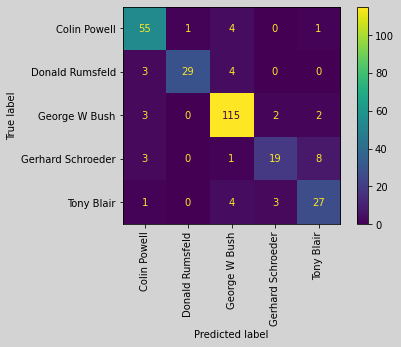
The Next Step
You just developed an autoencoder that can create an approximate representation of its inputs. You also used its latent representation to develop a classifier and applied it to a face recognition problem. While this may not be the best example to demonstrate the merits of the autoencoder as a supervised classifier, it should give you a fairly good idea of how to implement an autoencoder model and use its latent space representation for other tasks.
Now that you have a basic understanding of the autoencoder model, you can develop more advanced variants, such as a variational autoencoder or sparse autoencoder.
You can run the entire code shown in this tutorial in Google Colab or download the Python notebook here.
Learn More
Popular
Dive in
Related
Blog
How Waymo Is Using ML to Build a Scalable, Autonomous ‘Driver’
By Johanna Ambrosio • Jan 4th, 2022 • Views 5.5K
Video
How to Build an Effective AI Strategy for Business
By Catherine Williams • Oct 6th, 2021 • Views 4.5K
Video
How to Build an Effective AI Strategy for Business
By Catherine Williams • Oct 6th, 2021 • Views 4.5K
Blog
How Waymo Is Using ML to Build a Scalable, Autonomous ‘Driver’
By Johanna Ambrosio • Jan 4th, 2022 • Views 5.5K