How to Implement NLP Preprocessing Techniques in Python

Most of the textual data that we encounter in day to day life is unstructured. It has to be preprocessed, cleaned, and converted to a numerical format for input to a machine learning algorithm. So what’s the best way to do that?

In A Guide to Text Preprocessing Techniques for NLP, I discussed the basics of the text preprocessing pipeline. Here I'll focus on how to use various methods for the numeric representing and transformation of text data using Python. I’ll cover the following:

1. Text cleaning and dictionary construction in Python.
2. Representing a text document using a vector of statistical metrics.
3. Bag of words (binary and count based).
4. Term frequency.
5. Inverse document frequency.
6. Term frequency-Inverse document frequency.
7. Conversion of text documents to vectors of statistical metrics in Python.
8. Representing a text document using embedding matrices or vectors in Python.
9. Random embeddings.
10. Sinusoidal embeddings.
11. Loading pre-trained embeddings.

You can use these methods for further clustering, classification, labeling, or other tasks involving text data. (Note: You can also run the code in this article on Colab or download it from Github).

The Import Section

Let’s start by adding the following import section to the code. The inline comments explain the main purpose of the imported library.

A Note on Terminology

Below I will illustrate some algorithms and methods using a toy example as well as the 20 newsgroup text dataset. I’ll be using the following notations:

1. Text Corpus: The entire text used in the preprocessing and training stages. A text corpus comprises multiple documents.
2. Document: A set of sentences, grouped into a document. A document can be a single news item, an entire book, a magazine, a single email, or just a simple sentence.
3. Token/Word: A word of the English language. It is the smallest meaningful entity that we’ll process.
4. The prefix toy: All variables related to the toy example with just two documents are prefixed by the word toy.
5. The prefix docs: All variables related to the Newsgroup dataset are prefixed by the word docs.

Also note that the output you see in this tutorial won’t necessarily match the output you’ll get because of the random/stochastic nature of the algorithms involved.

The Newsgroup Dataset

The scikit-learn library includes the 20 newsgroup text dataset that consists of around 18,000 newsgroup posts, each corresponding to one of 20 newsgroup topics. This dataset can be used for several tasks, such as document clustering, document labeling, or document classification. I’ll use this dataset to illustrate how you can convert sentences to sequences of numbers, and further convert these sequences to word embeddings. For now, two categories are sufficient to show these methods, so I am loading only the documents from the alt.atheism and comp.graphics categories.

The code below reads the training subset using fetch_20newsgroups(), and prints some statistics. An example document is also printed below.

The corresponding output:

Cleaning Text and Creating a Dictionary With TextVectorization Layer in Keras

One of the first steps involved in text-processing is text cleaning, which can involve the following:

1. Convert the text to lowercase.
2. Strip the text of its punctuation.
3. Split the text into a sequence of tokens. (For the purposes of this tutorial, we’ll consider a single word to be a token.)
4. Build a dictionary of unique words.
5. Replace each word with its corresponding dictionary index.

Fortunately, the Keras library comes with a layer called TextVectorization that does all this in just one function call. Earlier TensorFlow versions came with a Tokenizer class that could be used to carry out all these tasks. However, this class is now deprecated so you should use the TextVectorization layer instead.

You can initialize the TextVectorization layer by specifying a standardize parameter. By default, the value of this parameter is set to lower_and_strip_punctuation. This implies that, by default, the layer will automatically convert the input text to lowercase and remove all punctuation from it. Another important parameter, split, with a default value of whitespace, tells the TextVecorization layer to split text based on whitespace characters. For more complex tasks, you can build ngram models using the ngrams parameter.

To help you understand the TextVectorization layer, I have taken a small toy example of a text corpus with just two documents. The code below shows the following:

1. TextVectorization() initializes the TextVectorization layer with output_sequence_length and max_tokens argument. The output_sequence_length specifies the length of the output vectors and max_tokens specifies the maximum dictionary size to use. The rest of the parameters are set to their default values, and hence we don’t need to specify them.
2. The adapt() method learns a dictionary from the text corpus.

The code also prints the entire dictionary and the sequence of numbers representing the toy corpus; each number being an index of the created dictionary. You can see that the different versions of the word ‘yourself’ written with mixed case are all automatically converted to their equivalent lowercase representation.

Note that the TextVectorization layer always adds an additional token, UNK, which stands for unknown token, to the dictionary. UNK is used to denote words not in the dictionary. Also, UNK replaces missing data in the dataset.

The corresponding output is:

Converting Newsgroups Text Corpus to Numbers

We can now convert the Newsgroups dataset to a sequence of numbers as shown below. The TextVectorization layer converts each document to a fixed-size vector. Documents shorter than this fixed size are padded with zeros.

The code prints the size of the dictionary along with an example of a document and its corresponding vectorized version. You can see that the input document has a lot of punctuation characters, extra spaces, and line-break characters. All of these are automatically filtered by the TextVectorization layer.

The corresponding output is:

Converting Words to a Numerical Statistical Representation

One possible method of converting textual data to numbers is to replace each word with a single number representing its importance or statistical weight in the document. You can calculate this importance weight by carrying out a statistical analysis of the words in individual documents as well as the entire corpus. In this technique, each document is replaced by a vector of numbers, where each vector component represents a unique word in the dictionary and the vector component’s value is the importance weight. Hence, the size of this vector is equal to the total unique words in the dictionary. In this representation, the order of words in the sentence is not taken into account.

What is a Bag of Words Representation of a Document?

As its name suggests, a bag of words representation treats a text corpus as a bag. Throw all the possible unique words of the corpus in the bag, and you have a bag of words representation.

The bag of words representation for a single document can be binary, i.e., each word can have a zero or one associated with it. A zero means the word didn’t occur in the document, and a one means it did occur. Each word can also be represented by its frequency. So the number associated with each word represents the number of times the word occurred in the document.

$f(w,d) =\text{count of word $w$ in document $d$}$

What is the Term Frequency Representation of a Document?

The count of a word in a document, being an absolute measure, may not be a good way to represent its importance. For example, compare a shorter document in which a word occurs many times against one with a longer document in which the same word occurs rarely. Both the word counts in the shorter and longer documents can turn out to be the same, but the relative importance of the same word in both documents is different. Hence, term frequency (TF) measures the relative frequency of a word in the document. It is defined as:

$\text{tf}(w,d) = \frac{f(w,d)}{n_d} = \frac{\text{count of word $w$ in document $d$}}{\text{total words in $d$}}$

There are also alternative definitions of TF in the literature, where the value of TF is logarithmically scaled as:

$\text{tf-scaled}(w,d) = \log(1+f(w,d))$

Note that the scaled version is taking into account only the absolute value of the frequency of the word and not its relative frequency. It just log scales the count of occurrence of the word in the document.

What is Inverse Document Frequency?

The Inverse Document Frequency (IDF) is a numerical measure of the information provided by a word. To understand this measure, let’s look at its definition:

$\text{idf}(w) = \log \frac{N}{t_w} = \log\frac{\text{total documents}}{\text{total documents that contain word $w$}}$

To avoid a division by zero, the above expression is often modified as:

$\text{idf}(w) = \log \frac{N}{t_w + 1} = \log\frac{\text{total documents}}{\text{total documents that contain word $w$ + 1}}$

Since log(1) = 0, the IDF of a word would be zero, if it occurs in all of the documents. However, if a word occurs in only a few specific documents, then the IDF is important to distinguish this set of documents from the rest. Hence, the IDF measure is designed so that a word is assigned high weights if it occurs in only a few documents of the text corpus. The IDF would be close to zero for words that occur in all or most of the documents of the corpus.

The IDF of a word provides a great numerical measure for identifying stop words in a document. Words like the, and, or, is, etc. are likely to occur in all of the documents and so their IDF would be zero. Words with a low IDF do not serve as helpful entities in classification and clustering tasks, and therefore can be removed from the corpus at the preprocessing stage.

On the other hand, physics terms are likely to occur only in scientific documents and not in documents related to politics or religion. Hence, the IDF of physics terms is likely to be high for a text corpus consisting of documents from diverse domains.

Note that the IDF of each word is computed globally from the entire corpus. Unlike TF, it does not depend upon a specific document.

What is Term Frequency-Inverse Document Frequency of a Word?

The Term Frequency-Inverse Document Frequency (TF-IDF) of a word in a document depends upon both its TF and IDF. High-frequency words in the document are important when computing the importance of a word, but they should not be considered if they occur in all documents. Hence, the measure TF-IDF is defined to assign a weight to each word according to its IDF, given by:

$\text{tfidf}(w,d) = \text{tf}(w,d) * \text{idf}(w)$

How is TF-IDF Computed in Keras TextVectorization Layer?

TF-IDF is computed differently in different machine learning packages. As there are varying definitions of TF and IDF in the literature, you can end up with different TF-IDF scores for the same word using different libraries. In Keras, TF-IDF is calculated by the TextVectorization layer as:

$\text{tfidf}(w,d) = f(w,d)\log\big(1+\frac{N}{1+t_w}\big)$

Example Computations of Different Metrics

In the toy corpus:

Document 1: be yourself, trust yourself, accept yourself

Document 2: be positive, be good

The word ‘be’ occurs in both documents, reducing its overall importance. The word ‘yourself’ occurs many times only in the first document, increasing its importance.

Taking the document d as: Be yourself, trust yourself, accept yourself, we have the following vector representations for it. Each row is a possible representation of the word given in the column.

Table 1: Different document representations using statistical measures.

How to Convert Documents to Numeric Weight Vectors in Python

The TextVectorization layer can be set up to return various numeric statistics corresponding to different documents of the text corpus. You can specify different constants for output_mode to compute bag of words or TF-IDF vectors as shown in the code below. A little manipulation is required for the relative frequency matrix.

The corresponding output is:

Word Embeddings: A Vector Representation of Words

Another innovative method you can use to map text to numbers is to replace an individual word with a vector, where a vector is a list of real numbers. This representation of a word as a vector is called the embedding vector. The embedding represents or encodes the semantic meaning of a word. Hence, two similar words will have two similar representations. The great thing about this method is that you can use simple mathematical operators, e.g., the dot product to determine the degree of similarity between different words. Examples of these embeddings include word2vec and GloVe, both for finding associations between different words.

Here are some of the possible word embeddings.

Initializing Word Embedding to Random Numbers Using Keras

Keras includes an Embedding class in its library that converts positive integer indices of words to dense vectors with random values. You can then use this layer to learn a word embedding during model training or to define a subclass of Embedding class to define your own embedding. Let’s look at this class in action on our toy example:

The toy_vectors and toy_embedded_words are shown in the annotated figure below:

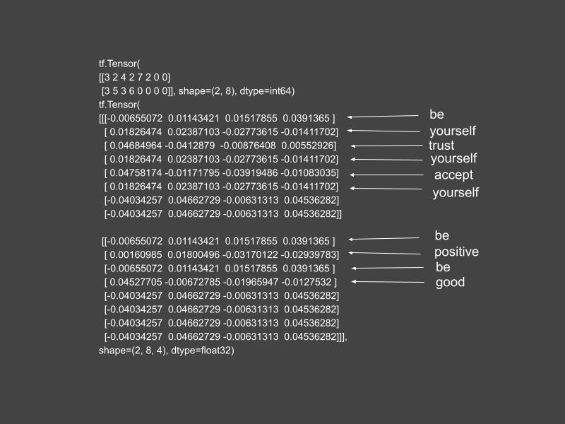
Figure 1: Random embedding of toy corpus. Source: Mehreen Saeed

The word embeddings are just a jumble of numbers that are hard to comprehend. However, you can view these embeddings as an image in Python as shown below. Both sentences have a different random signature.

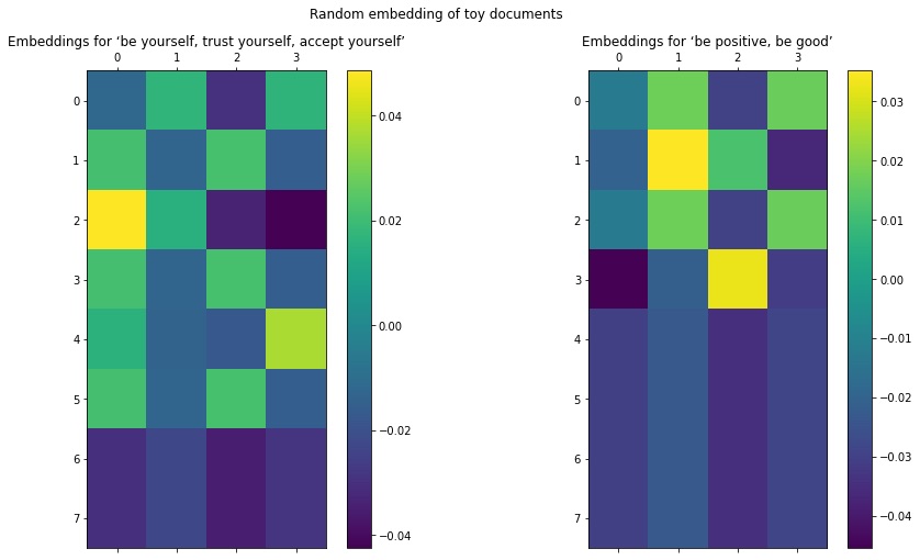
In the graphic on the left, you can see that rows 1, 3, and 5 represent the word ‘yourself,’ and therefore are all the same. The same goes for the word ‘be’ as shown in rows 0 and 2 of the figure on the right.

Next, let’s look at the random embeddings of the two documents of the Newsgroup corpus that we loaded earlier. I have chosen these two documents arbitrarily.

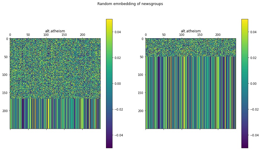
You can see that the first half of both embeddings matrices are random pixels. The stripes in the bottom half show the zero padding of the matrices. If you use this layer in a machine learning model pipeline, TensorFlow automatically learns the embeddings according to the training data. The image below shows how word embeddings are learned when training a transformer.

Figure 2: Random and Learned Embeddings.

Word Embeddings in Transformers: Attention is All You Need

One possible word embedding is described by Vaswani et al. in Attention is All You Need, a seminal paper describing the transformer model. The authors convert a sentence corresponding to a sequence of words to an embedding matrix based on the sinusoid functions. An input sequence of length L is mapped to a place in the row i of the embedding matrix using the function P given by:

$P(i, 2j) = \sin\big(\frac{i}{n^{2j/d}}\big)\\$$P(i, 2j+1) = \cos\big(\frac{i}{n^{2j/d}}\big)$

Here:

i: Index of a word in the input sequence, 0≤i<L.

j: Used for mapping to column indices with 0≤j<d/2. In the expression 2j or 2j+1 distinguishes an even index from an odd index.

d: Output embedding dimension or the number of columns of the embedding matrix.

j: Index of the output embedded vector.

P(k,j): Function that maps an index k in the input word sequence to index (k,j) of the output matrix. The even indices are mapped using a sine function and odd indices are mapped using a cosine function.

n: Constant defined by the user. Its value is arbitrarily set to 10,000 by the authors of “Attention is All You Need.”

As the position of every word in a sequence is important, the preprocessing layer computes two embedding matrices. One matrix represents the word embeddings and the other represents an encoding of positions. The goal of the latter is to add positional information to the words. In this way, each sentence will have the same corresponding positional matrix but a different word embedding matrix. The final word embedding matrix input to the transformer is a sum of word and position embeddings.

Implementing Word Embedding in Python with Keras

Keras does not have a built-in method or layer to give you the sinusoidal word and position mapping. However, it is easy to write your own class that computes these embeddings. The code below shows how you can create your own MyEmbeddingLayer class by subclassing the Keras Layer. Following are a few important features of this class:

1. The get_encoding_matrix() method computes the encoding matrix from the sine and cosine functions.
2. The embedding_layer_words attribute defines an embedding layer with the weights parameter specifying the encoding matrix and the trainable parameter set to False. This layer will automatically take a word sequence and map it according to the specified weights (embedding_matrix_words).
3. The embedded_indices attribute holds the embedding matrix for the position indices. As all sentences have the same position embeddings, you can store this matrix at initialization time.

Let’s view the embeddings for the two toy sentences. To give you a better idea of this embedding, I have increased the size of the sequence length by using pad_sequences(), and increased the output dimension to 30 before rendering the embeddings as an image.

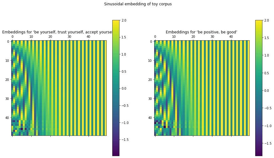
Next, let’s view the sinusoidal embeddings of the Newsgroups text. Here, I arbitrarily chose two documents to embed. Notice that the embeddings of both documents are different, giving them a unique signature.

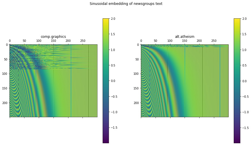
Retrieving a Pre-Trained Embedding in TensorFlow

TensorFlow Hub, a repository of pre-trained models that you can use in your project, also contains a collection of text embeddings trained on different types of problems. It is a great resource if you don’t want to spend time building or learning your own embeddings from scratch, and you also have the option of transfer learning by loading a pre-trained embedding and tuning it for your specific application.

In the example below, I have loaded the Universal Sentence Encoder model that has been trained on a large dataset from different sources, and can be used to solve various NLP tasks. This model converts an input word, sentence, or an entire document to a one-dimensional vector of embeddings.

You can explore various TensorFlow pre-trained embeddings and choose the one right for you. Effectively, all of these models have been built using the same protocol, so if you understand this example you’ll better understand how to work with other pre-trained word embeddings in TensorFlow Hub.

The code below transforms the documents from alt.atheism and comp.graphics categories to their respective embeddings using the Universal Sentence Encoder model. Both embeddings are rendered as images. One row of the image represents one newsgroup document.

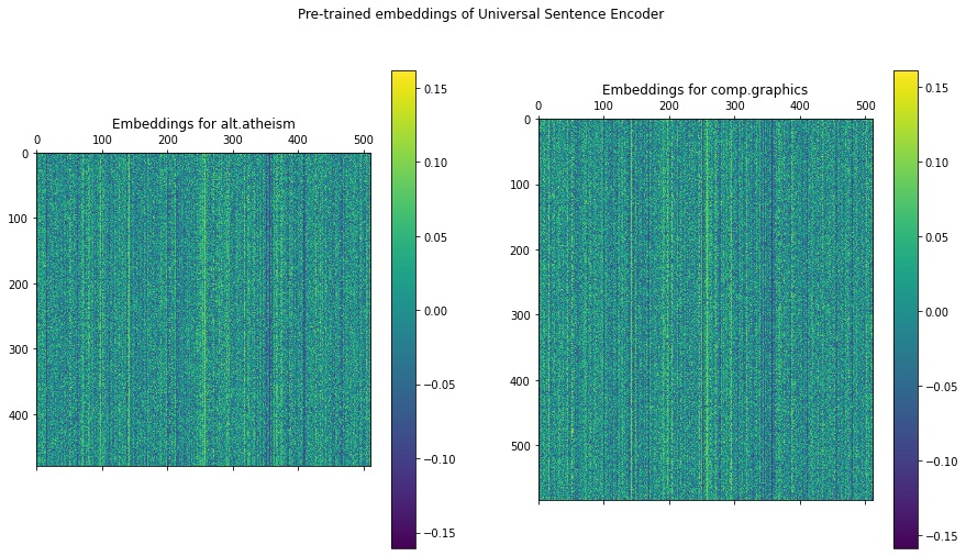
Unlike random embeddings, you can see that the learned embeddings loaded from the Universal Sentence Encoder are much smoother. If you look closely enough, you’ll notice that they are also different from each other for both Newsgroup categories.

Correlation Between Documents

To get an idea of the merits of learned embeddings of the Universal Sentence Encoder, look at the correlation between different documents. We expect correlations between documents of the same category to be high, and the correlation of documents between two different categories to be close to zero.

While correlation values range from -1 to +1, I am taking their absolute value to approximate the magnitude of similarity between the documents from alt.atheism and comp.graphics. Also, printing the correlation values is of no use to us as it is simply a jumble of numbers. Instead, we render them as an image as shown in the code below.

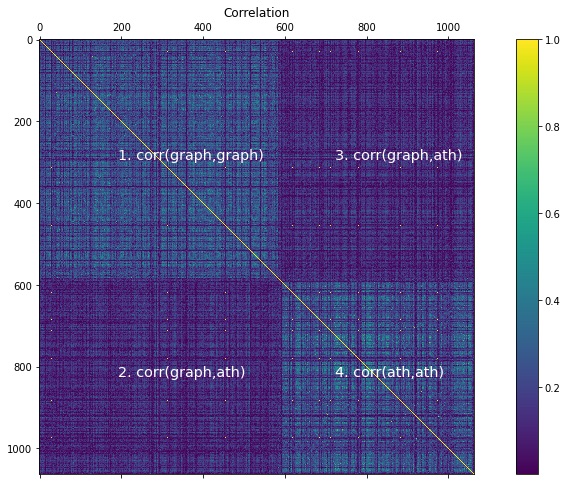
In the correlation matrix above, the yellow diagonal represents the correlation of a document with itself, and has the maximum value of one. Also, there are four sub-matrices (labelled in the figure) for:

1. Correlation between documents of alt.atheism with documents of alt.atheism
2. Correlation between documents of comp.graphics with documents of alt.atheism
3. Correlation between documents of comp.graphics with documents of alt.atheism
4. Correlation between documents of comp.graphics with documents of comp.graphics

The correlations between documents of alt.atheism with correlation of documents from alth.atheism is close to zero, as indicated by the dark blue color. However, the correlation between the documents from the same categories has many lighter tones that indicate greater than zero values. While some documents within the same category have low correlations, the overall matrix shows a clear discrimination between the two categories of newsgroups.

What’s Next?

So far you've learned the first steps for converting text to a format that can be used for further processing by a machine learning or pattern recognition algorithm. Understanding various text preprocessing techniques, including statistical metrics of text and word embeddings, is important for developing all types of NLP applications. How you preprocess text and the text representations you use will significantly affect the performance and accuracy of your end application. Now you are ready to set up your own NLP pipeline for the task at hand.

Learn More

1. A Guide to Text Preprocessing Techniques for NLP
2. How to Build a Transformer for Supervised Classification